Terra Sulis worked with Friends of the Earth to create the Tree Canopy Map using LiDAR data from the Environment Agency’s National LiDAR Programme. The LiDAR (Light Detection And Ranging) system uses a laser to accurately measure the distance between the active-sensor and the target below. The system collects millions of point locations in 3D space. These data are then processed by the Environment Agency (EA) to generate a set of values for each square metre across all of England. This is a vast data set. Within any square metre, photons from the laser may be reflected from a variety of locations within the vertical column between the sensor and the ground. Anybody can download the EA data but processing it at the national level is a big undertaking.
Objective
The main objective of the project was to produce a detailed map of England’s trees using the Environment Agency National LiDAR Programme data. To achieve this we developed a computer algorithm to process the LiDAR data and identify trees in a reliable way, whilst excluding non-tree objects. It is not possible to do this with 100% accuracy but we aimed to minimise both false positives and false negatives. As well as producing detailed trees maps for the whole of England, aggregated area measurements were compiled at the Local Authority, LSOA and Ward levels.
Data Inputs
The primary data input was the Environment Agency’s National LiDAR Programme Data, consisting of:
- First Return, FZ – the first LiDAR height return from the given 1 m x 1 m cell
- Digital Surface, DSM – the last LiDAR height return from the given 1 m x 1 m cell
- Terrain, DTM – the terrain surface height
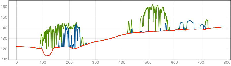
The example above includes the ground surface in red, buildings and some tree trunks in blue and tree canopy in green. This is a simple example which contains no noisy features such as buses, pylons, gas tanks, etc.
In addition, other ancillary data sets were utilised from the Ordnance Survey open-data sources, including:
- Building footprints
- Motorways
- Railways
- Glasshouses
- Power transmission lines
- Tidal water
- Surface water features
Google Maps was used as a reference during development but not as an input data set.
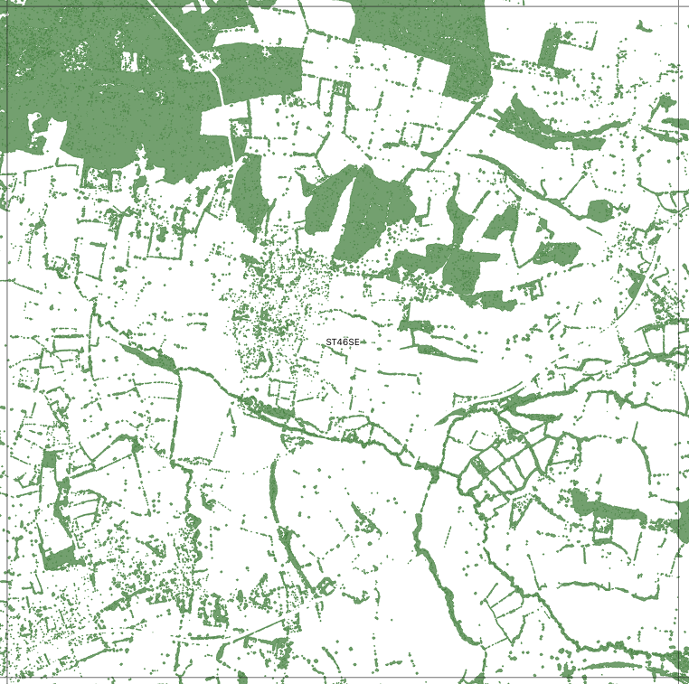
The example above is for OS block ST46SE which is 5km x 5km in size. There are approximately 5,500 such data blocks across England. The processing is done in such a way that features are identified across block boundaries to form a seamless map across blocks.
Algorithm Approach and Summary
An algorithm that identifies trees from the LiDAR data has been developed in Excel and implemented using bespoke Java procedures, Postgres and QGIS.
The algorithm has two main components, referred to as the “negative” and “positive” models.
The negative model seeks to identify objects that are not trees, for example buildings and areas of flat ground. It also filters out anything with a height below 3m, which is considered the minimum height for a tree. Furthermore, areas of water and some other exclusion categories are filtered out.
The negative model identifies the ground by looking at the difference between the height of the ‘First Return’ signal and the height of the ‘Terrain’. It then expands the ground area in any direction of low gradient, for example up ramps and driveways. It then draws an edge line around all the non-ground objects (see Figure 1 of St Pauls in London).
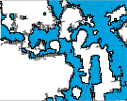
Figure 1. – Ground (blue) and Edges
After the ground and edges are identified, a buildings model is run. This uses both the LiDAR data and the Ordnance Survey buildings layer to identify buildings. The outlines are smoothed using spatial filters (Figure 2).

Figure 2. – Buildings
Once the areas of ground, buildings and other non-tree categories have been excluded, the positive model looks at the remaining areas and identifies pixels that are likely to represent trees. To do this we calculate 10 statistical factors for each pixel. These include the gradient, the height, variability of direction, and translucency. We also look at the range and standard deviation of a selection of these measures.
The model has been ‘trained’ by looking at a variety of data samples which we know to represent trees. A thresholding process has been used to establish ranges of values for the 10 statistical factors.
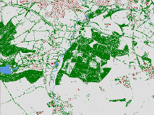
Figure 3. – Algorithm output – Longleat, green trees, red buildings
The algorithm has been implemented using the Java programming language and Postgres relational database to manage the large number of input files. It processes each tile of LiDAR data, first running the negative exclusionary model and then uses the positive model to look for pixels where the tree thresholds are met (Figure 3).
Data Processing Considerations
The EA LiDAR data are arranged into 5 km x 5 km tiles, of which there are approximately 5,500. There are tens of thousands of ancillary files. Processing these tiles is a very computer intensive process which is complicated by the need to take into account the adjacent areas in neighbouring tiles. It is necessary to take account the neighbouring tiles to ensure continuity across the tile boundaries.
Outputs
The outputs are:
More than 5,500 raster tiles with “tree” pixels
To aid data management and ease of use the raster tiles have been vectorised and dissolved together into large 25 km x 25 km tiles, of which there are 275 tiles.
An examples of a 25km tile is shown below, together with the Open Street Map equivalent.
| 25 x 25 km tile with 5x5km tile grid | Open Street Map of the same block |
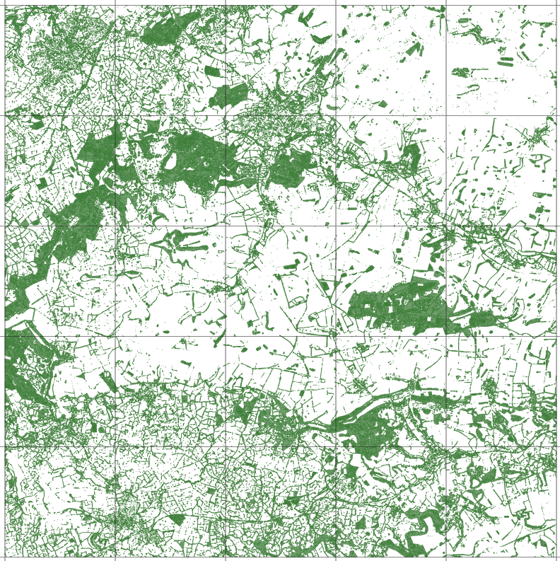 | 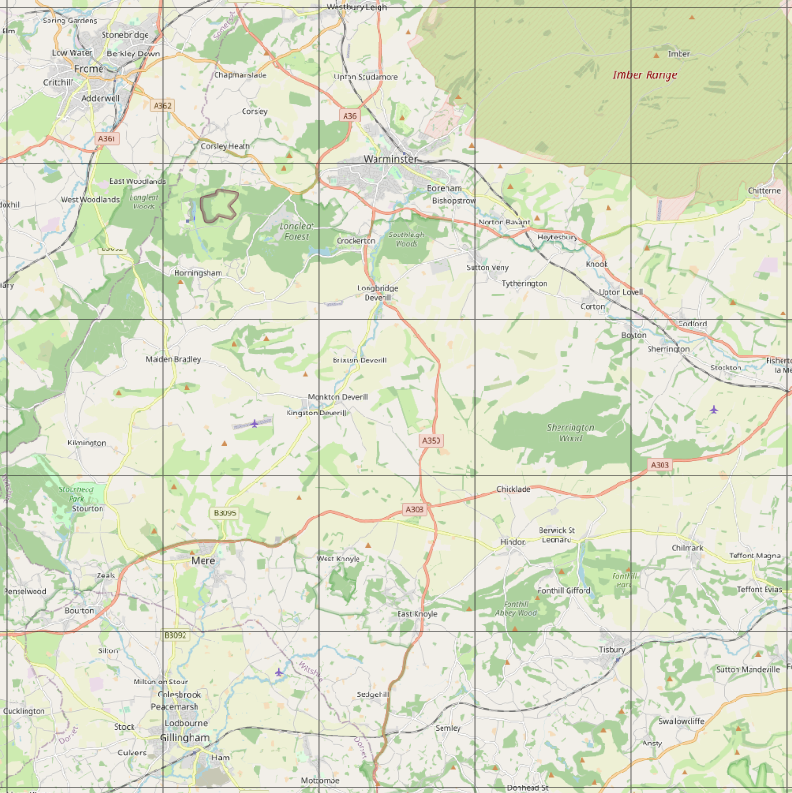 |
Data Availability
The data set are no longer available. However you can still access the web map version at Friends of the Earth.
Area Based Aggregations
This is a very large data set and it is useful of aggregate the data by administrative units, LSOA, Ward, Parish, etc. You can find aggregation of the data by LSOA (Lower Super Output Area) on the Friends of the Earth website. Other aggregations, including wards, are planned.